Designing a 10K-GPU IB Compute Fabric: Six Decisions That Fix the Topology

In one sentence: a 10K-scale network is not "buy a pile of switches and cables and plug them in". It is six decisions made in sequence — how many ports per GPU, two or three tiers, what oversubscription, how to align rails, how big a POD should be, and where the control plane sits. Once these six are settled, the topology is essentially unique.

This article is about the design method, not the line-by-line breakdown of a single diagram. The diagram appears once, at the end, as the finished product of all six decisions — the real shape of 1,250 HGX H100 nodes. If you want to walk the port accounting and packet hops of that diagram tier by tier, see the companion piece A 10K-GPU InfiniBand Parameter Plane: 3-Tier Fat-Tree with 1,250 HGX H100 Nodes.

The six decisions at a glance

Step	Decision	Criterion	Value in this example
1	How many 400G ports per GPU	Training vs. inference workloads	1 GPU : 1 port
2	Two or three tiers	Endpoints as a multiple of switch radix	Three tiers (313 Leafs > 64 ports)
3	Oversubscription	Workload shape + budget	1:1 non-blocking
4	How to align rails	Mapping of GPU index to NIC and Leaf	8 rails, aligned by GPU index
5	How to size PODs	Failure / cabling / scheduling domains	5 PODs (4×256 + 1×226)
6	Where the control plane sits	SM / UFM high availability	UFM pair + active-standby SM

1. Separate the three planes first — do not mix storage and management into the compute fabric

A GPU cluster never has just one network:

• Compute plane (parameter plane): GPU-to-GPU traffic — NCCL All-Reduce, All-to-All and MPI. This is InfiniBand's home turf and the subject of this article.
• Storage plane: parallel file systems (Lustre / GPFS) or object storage, typically a separate IB or RoCE fabric with its own Leaf/Spine.
• Management plane: out-of-band BMC, provisioning, monitoring, and the heartbeat traffic of the subnet manager (SM) and UFM.

The three planes must be isolated physically, or at least logically (PKey / SL, or dedicated physical ports). The reason is that three kinds of traffic cannot coexist: training traffic is extremely latency-sensitive; storage traffic is long-lived, large-block bursts; management traffic must never break because training traffic congested the fabric — once the SM loses contact with the switches, the whole network loses its routing. This is the root cause of many "small clusters run fine, big clusters keep breaking" stories: the hardware is fine; three classes of traffic were squeezed onto one fabric.

2. Decision one: how many 400G ports per GPU

This is the most expensive decision in the design, and the hardest one to reverse.

An HGX H100 baseboard carries 8 GPUs with 8× 400G cluster ports (four dual-port ConnectX-7 mezzanine cards). Eight GPUs, eight ports — 1 GPU : 1 port by construction, with 8×400G = 3.2 Tb/s per node to the fabric. If you instead design for two GPUs sharing one port, injection bandwidth is cut in half, and so is the theoretical All-Reduce ceiling — and that "half the ports" saving usually only removes Leaf ports and a smaller set of optical modules, in exchange for every iteration running at half speed.

The criterion is straightforward:

• Pretraining / large-scale fine-tuning → 1 GPU : 1 port, no port oversubscription at all;
• Inference-first → 2 GPUs : 1 port or even less is acceptable, because inference traffic is request-level and sparse rather than a synchronization barrier;
• Mixed workloads → size it by queue mix; give training full bandwidth and constrain inference jobs to a lower-bandwidth partition at the scheduler level.

For this example: 1,250 nodes × 8 ports = 10,000 × 400G endpoints, an aggregate injection capacity of 10,000 × 400 Gb/s ≈ 4 Pb/s. Pin this number down first — it is the baseline for every tier ratio that follows.

3. Decision two: derive the tier count from radix, not from instinct

The number of tiers is not a guess; it is arithmetic. On a k-port switch, a 1:1 non-blocking design can dedicate only half the ports downward to endpoints and half upward to the next tier:

Endpoints per Leaf = k / 2
Total Leafs        = N / (k / 2)
If total Leafs > k → three tiers required (add Core / super-spine)

Plug in a 64-port NDR switch (k = 64):

• Each Leaf accepts at most 32 endpoints (the other 32 ports face up);
• 10,000 endpoints → 10,000 / 32 = 312.5 → round up to 320 Leafs;
• 320 > 64 → three tiers are mandatory.

This gives a useful rule of thumb: with 64-port switches at 1:1, a two-tier fabric tops out at 64 × 32 = 2,048 GPUs. That is where the "2,048 GPUs is the two-tier ceiling" arithmetic comes from — and why a 10K cluster is almost inevitably a three-tier fat-tree, regardless of vendor preference.

A look at the next hardware generation: the 800G-era Quantum-X800 Q3400 has 144 ports, and 144 × 72 = 10,368 endpoints — a 10K cluster just fits back into two tiers. Removing one tier removes an entire layer of switches and a layer of optical modules, which is the single biggest cost lever in next-generation cluster design.

Note: round Leaf counts up in groups, not per device. In this example they come in groups of eight: 320 = 40 groups × 8. The grouping must line up with POD partitioning and rail numbering, or the cabling tables become unmanageable later.

4. Decision three: set oversubscription, and upgrade from "port accounting" to "bandwidth accounting"

Oversubscription has a one-line definition:

Oversubscription = total downlink ports / total uplink ports

A ratio of 1 means non-blocking — any two endpoints can run line rate; 2:1 means two downlink streams compete for one uplink, so at full contention each gets roughly half.

Oversubscription	Peak All-to-All bandwidth	Switch count	Fits
1:1	100%	Highest	Pretraining, large-scale parallelism, All-to-All-heavy (MoE)
2:1	~50%	~1/3 fewer	Fine-tuning, mixed workloads
3:1 ~ 4:1	25% ~ 33%	More than half fewer	Inference, small single-rack jobs

The most common design error is reconciling port counts without reconciling bandwidth: 10,240 downlink ports and 10,240 uplink ports on the Leaf layer look like a clean 1:1 on paper, but if half the uplinks land in the same Spine group, there are not enough equal-cost paths and queues build up at peak anyway. Real accounting has to land on three checks:

1. At every tier, downlink port count equals uplink port count (count);
2. At every tier, uplinks are spread evenly across every upper-tier group (distribution);
3. For any two endpoints, worst-path bandwidth equals a single port's line rate (paths).

In this example every tier has 10,240 ports at 1:1, and Leaf uplinks follow a group-to-group full mesh, so the first two checks hold; the third is confirmed during acceptance with a cross-POD All-Reduce test, see section 10.

5. Decision four: align rails — turn "8 GPUs, 8 ports" into 8 tracks

This is the step most often skipped, and one of the biggest movers in measured results.

Without rails, each server's eight ports are wired to whichever Leaf is convenient. With rail-optimized wiring: GPU0 on every node across the entire cluster goes to Rail 0 Leafs, GPU1 to Rail 1 … GPU7 to Rail 7, with each rail backed by its own Leaf group.

The payoff is shorter communication paths: NCCL's ring and tree algorithms do local aggregation within a rail first, so rail-local traffic crosses only the Leaf–Spine hop; cross-rail traffic has to climb higher. For an 8-GPU-node All-Reduce, this keeps a large share of traffic at two network hops.

The costs have to be acknowledged:

• Larger failure domains: a bad Leaf or optical module on one rail hits the same GPU slot on every node at once (for example, every GPU3). It looks like "the training framework crashed" when it is actually single-rail degradation;
• Strict cabling discipline: eight bundles per rack, one color or label per bundle. One misplugged fiber means "some GPU on one node is on the wrong rail", and the problem only surfaces under specific communication patterns — extremely hard to debug.

The supporting deliverable is a rail table (node → 8 ports → 8 rails → specific Leaf ports), kept as a handoff document. Acceptance and fault location both depend on it. For how this lands at 384-GPU scale, see Rail-Optimized Fat-Tree with 1.5:1 Oversubscription.

6. Decision five: partition PODs so most traffic never leaves the building

A POD is not just a group of racks. It is simultaneously a failure domain, a cabling domain and a scheduling domain. A good partition has most daily collective communication closed inside the POD, with only cross-POD data-parallel gradient sync climbing to the Core.

The partitioning criteria, in priority order:

1. Integer multiples of switch groups: a POD's Leaf count should be an integer number of groups × 8 devices, so group-to-group meshes stay clean;
2. Rack and power boundaries: POD edges should coincide with row-level power distribution so failure isolation is real;
3. Parallelism strategy: keep each data-parallel group inside one POD where possible, so All-Reduce stays local.

In this example, 1,250 nodes are split into 5 PODs: the first four hold 256 nodes each (2,048 ports / 64 Leafs / 8 groups), and the fifth holds the remaining 226 (not fully populated). In each full POD, 64 Leafs × 32 downlink ports = 2,048 ports, matching 256 servers × 8 ports one-for-one — no spare port and no missing port.

7. Decision six: the control plane decides whether this network is operable

Once the hardware is laid, the network's "brain" is the subnet manager.

• Active-standby SM: exactly one primary SM computes LIDs and routes, with one standing by. SM failover at 10K scale must be rehearsed, not just documented.
• UFM pair: the two UFM servers on the right of the diagram are the control plane — topology discovery, port health, error counters and fault location. If one fails, the other takes over.
• SHARP: Quantum-2 supports SHARPv3, which can perform All-Reduce reduction inside the switches and cut communication volume. It is an explicitly-enabled feature, off by default; many clusters buy SHARP-capable switches and never turn it on.
• PKey / SL: isolate compute and storage planes with separate PKeys; map compute traffic to a high-priority VL so training is protected first under congestion.
• Adaptive routing: enable it by default; combined with credit-based flow control it protects tail latency above 80% load.

One quick LID capacity check: IB LIDs are 16-bit, with roughly 49,000 usable under a standard OpenSM configuration — comfortably enough for 10,000 endpoints and close to a thousand switches. The real concerns are routing table size and SM convergence time, not LID count.

8. The result: a three-tier fat-tree for 1,250 HGX H100 nodes

With all six decisions settled, the shape is: a three-tier fat-tree with 320 Leafs (40 groups × 8), 320 Spines (40 groups × 8), 256 Core switches (8 groups × 32), 1,250 eight-GPU servers, and two UFM nodes as the control plane.

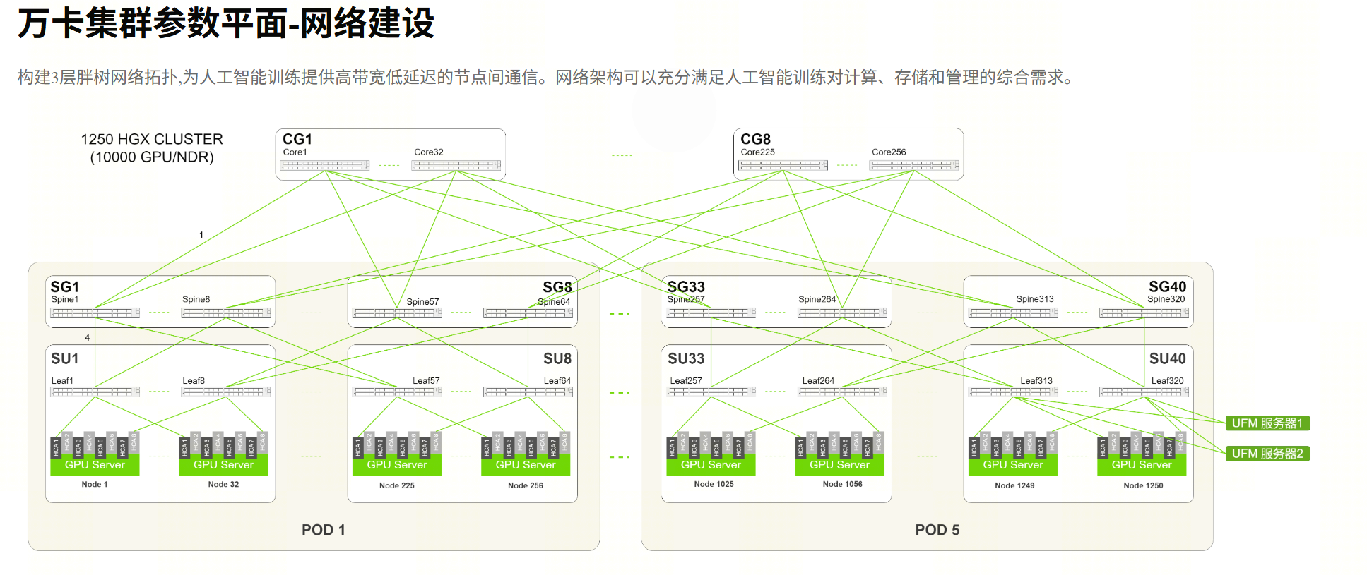
Port accounting, read back from the diagram:

Tier	Count	Ports/device	Down / up	Conclusion
Endpoints	1,250 nodes × 8 ports	400G	10,000 injection ports	1 GPU : 1 port
Leaf	320 (40 groups × 8)	64	32 down + 32 up	10,240 ≥ 10,000, 2.4% headroom
Spine	320 (40 groups × 8)	64	32 down + 32 up	10,240 ↔ 10,240, 1:1
Core	256 (8 groups × 32)	64	40 to Spine + 24 inter-group	40 × 256 = 10,240, 1:1

One trade-off to confirm up front: each Core switch has 64 ports, 40 facing Spines and about 24 left for inter-group meshing. Read back from the diagram, inter-group capacity is roughly 256 × 24 = 6,144 ports, about 0.6:1 against 10,240 injected. In other words, intra-POD and near-POD paths are strictly non-blocking, but an All-to-All with all five PODs saturated simultaneously is not strictly 1:1 at the top tier.

This is not a defect; it is a trade-off. Full 1:1 inter-group meshing requires another tier or higher-radix switches, and the cost jumps sharply. The correct handling is to make it explicit:

1. Write the 0.6:1 into the design document's oversubscription budget — do not discover it at acceptance;
2. At the scheduler level, keep jobs grouped inside PODs (data-parallel groups stay within one POD, or span only a few);
3. During acceptance, run one dedicated five-POD All-to-All test and compare measured values against theory, so the number is known rather than guessed.

If your workloads are MoE-style with extremely heavy All-to-All, the top tier has to be re-priced: giving up 10% of the GPUs is preferable to letting the top tier become the bottleneck of the entire fabric.

9. Five design errors you are most likely to make

1. Port accounting instead of bandwidth accounting: pretty numbers, broken paths. Reconcile down to worst-path bandwidth.
2. A single SM: the SM is a single point of failure — when it dies, the fabric loses routing. Active-standby plus a failover rehearsal is a hard requirement.
3. Rails not aligned, no rail table kept: performance issues appear only under specific communication patterns, with nothing to debug against.
4. Optical module budget missed: at roughly ten thousand 400G ports, transceivers and cabling outside the switch BOM are often the bigger line item; 1,024-GPU NDR optical budgets routinely run into the million-dollar range. Establish the budget from port count × unit price before selecting vendors.
5. Storage and management squeezed into the compute plane: short-term hardware savings, long-term fabric-stability incidents.

10. Acceptance checklist before handoff

1. Physical layer: ibstat all green, port rate and width match the design, baseline error counters archived;
2. Single hops: run ib_write_bw / ib_read_lat at three distances — same Leaf, same Spine, cross-Core;
3. Topology consistency: audit 10% of the rail table against actual cabling — every misplugged fiber must be found;
4. Collectives: NCCL All-Reduce from one POD up to all five PODs; the bandwidth decay curve must match the oversubscription budget;
5. SHARP effectiveness: compare All-Reduce duration before and after enabling it — buying SHARP without turning it on is wasted money;
6. Control plane: rehearse SM failover and UFM takeover, recording switch time and business impact.

Three closing lines

• Fix injection at 1:1: one 400G port per GPU. Do not economize at this layer.
• Tier count comes from arithmetic: when Leaf count exceeds switch radix, three tiers are mandatory; higher radix can bring 10K back to two.
• Oversubscription follows the workload: non-blocking for training, oversubscribed for inference, ratioed for mixed — and write every trade-off into the document.

Once the design is done, what remains is construction and operations. And the first document of any construction project is always the port accounting table.

Further reading

• A 10K-GPU InfiniBand Parameter Plane: 3-Tier Fat-Tree with 1,250 HGX H100 Nodes
• Rail Topology + 1.5:1 Oversubscription: Design a 48-Node Cluster Like a 10K-GPU One
• IB Three-Plane Separation: PKey Partitions, SL/VL and IPoIB
• InfiniBand Performance Tuning for AI Workloads
• GPU Training Network Troubleshooting: Packet Loss, Congestion & NCCL Timeouts