A 10K-GPU InfiniBand Parameter Plane: 3-Tier Fat-Tree with 1,250 HGX H100 Nodes

In one sentence: this is not just a topology diagram — it is the communication backbone of a "10,000-GPU parallel computer". Following whole → parts → whole, this article breaks the IB parameter plane (1,250 HGX H100 nodes, 320 Leaf, 320 Spine, 256 Core) into engineering knowledge you can apply directly.

1. The Big Picture: What a 3-Tier Fat-Tree Solves

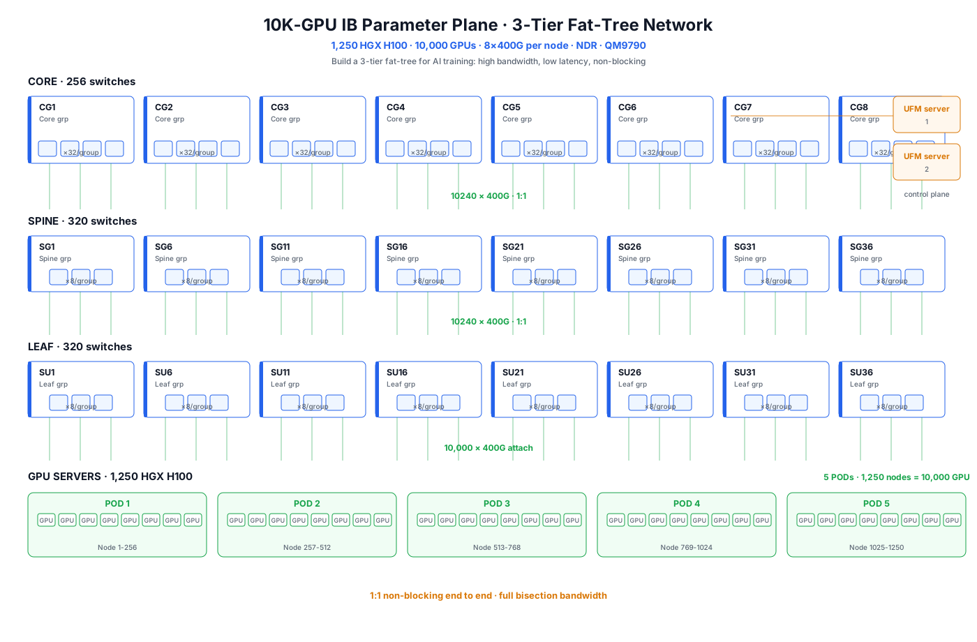
During AI training, GPU-to-GPU traffic has an extreme pattern: All-Reduce requires every GPU to exchange gradients at the same time, and All-to-All moves data between any two GPUs directly. The design goal of the communication network (parameter plane / compute fabric) is simple — no bandwidth degradation and predictable latency between any two GPUs. A 3-tier fat-tree (Core / Spine / Leaf) is the standard structure built for exactly this:

• Leaf tier: closest to servers, aggregates each node's 8×400G ports into the fabric;
• Spine tier: provides horizontal forwarding so any two Leafs have paths between them;
• Core tier: opens the whole network — cross-POD traffic converges and re-distributes here.

Key numbers: 1,250 × HGX H100 (8 GPUs each) = 10,000 GPUs, each node has 8×400G IB ports → 10,000 × 400G attachments; supported by 320 Leaf, 320 Spine, 256 Core switches — all NVIDIA Quantum-2 QM9790 (64-port NDR 400G, 51.2 Tb/s aggregate per switch).

2. Do the Math First: Why These Numbers Fit Perfectly

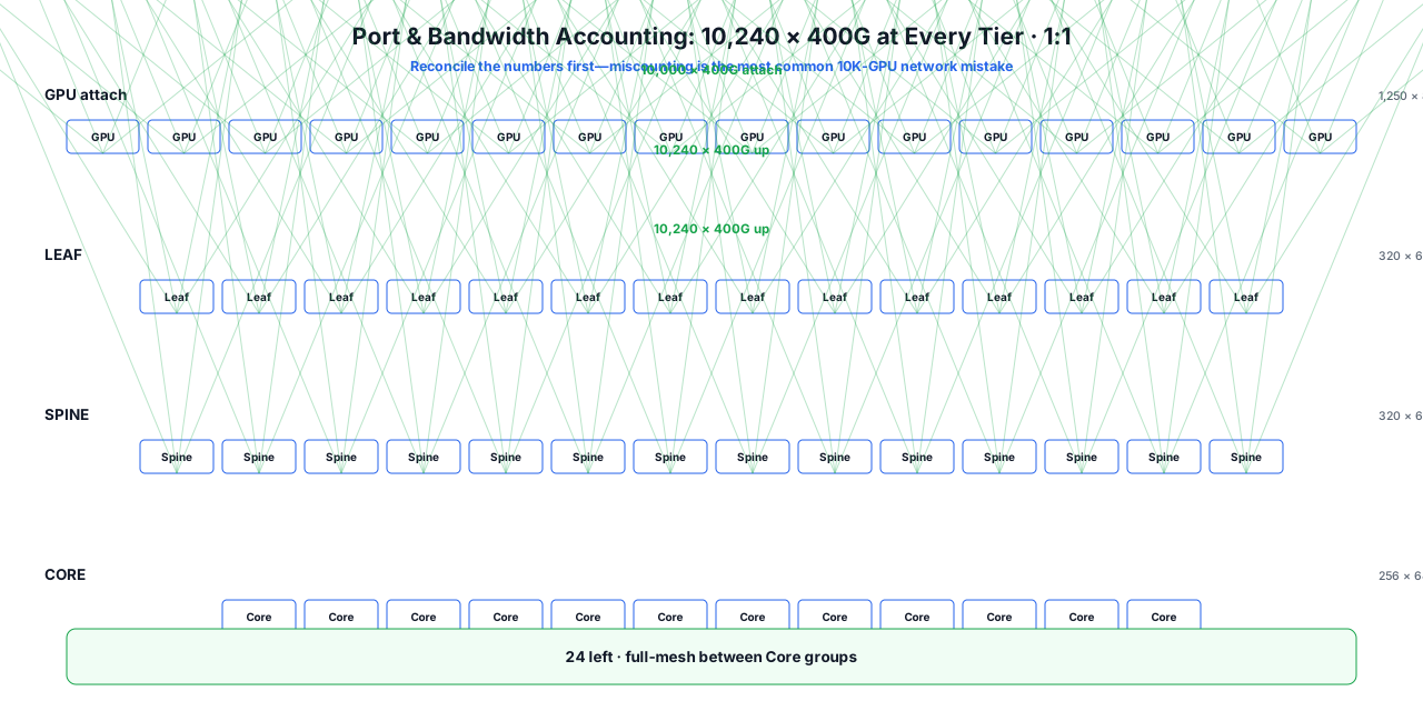
Before writing anything, reconcile the numbers — the most common mistake in a 10K-scale network is "the numbers don't add up".

Tier	Count	Ports/Switch	Total ports	Role	Check
GPU attach	1,250 × 8 ports	400G	10,000	1×400G per GPU	baseline
Leaf	320	64	20,480	32 down + 32 up	down 320×32 = 10,240 ≥ 10,000
Spine	320	64	20,480	32 to Leaf + 32 to Core	each side 10,240
Core	256	64	16,384	40 to Spine + 24 inter-group	to Spine 256×40 = 10,240

Key conclusion: Leaf → Spine → Core each carry exactly 10,240 × 400G ports — a 1:1 non-blocking fabric. Every GPU-to-GPU path keeps full bandwidth end to end. This is the essential difference from a general-purpose network: a business network may be oversubscribed (contended), but in a training fabric, 1% of oversubscription makes All-Reduce 1% slower.

One more note: each Core switch has 64 ports; 40 go to Spine and the remaining ~24 form a full-mesh between Core groups — this is why the Core tier never becomes a bottleneck at 10K scale.

3. From Whole to Parts: Inside a POD

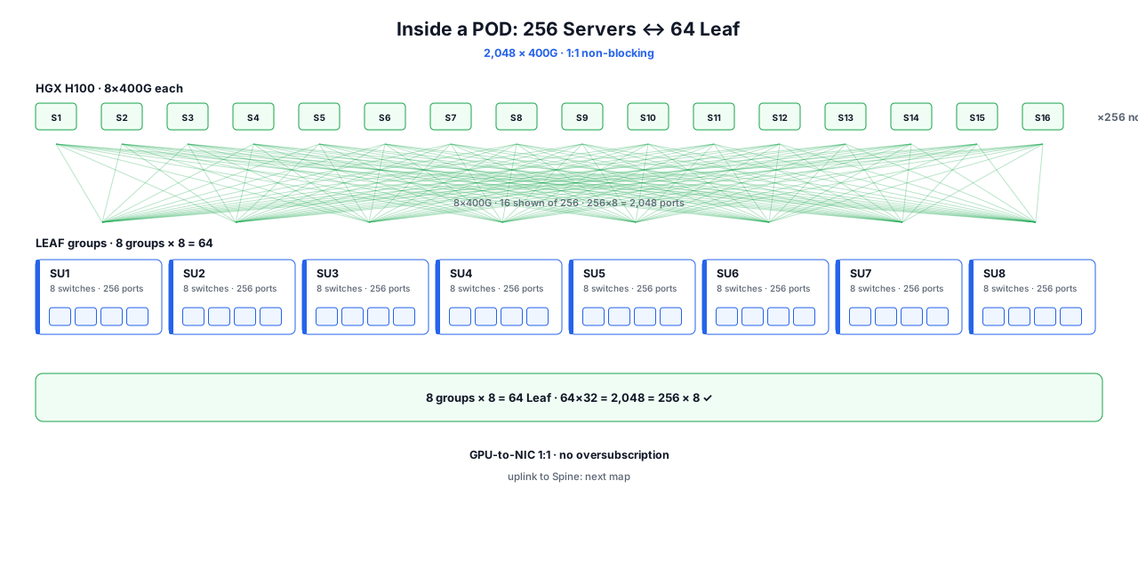
The fabric is divided into 5 PODs: the first four have 256 nodes each, the fifth has 226 — 1,250 total. Taking a 256-node POD as an example:

• 256 × HGX H100 × 8 ports = 2,048 × 400G ports;
• Served by 8 Leaf groups × 8 switches (64 Leaf total): 64 × 32 downlink ports = 2,048 — a perfect 1:1 match;
• One Leaf group (8 × 32 = 256 ports) connects exactly 32 servers (32 × 8 = 256).

Why 8 ports per server? On an HGX H100, each of the 8 GPUs owns a dedicated 400G ConnectX-7 NIC (two Cedar-7 mezzanine cards on board, 4 ports each). 8 ports = 8 GPUs, GPU-to-NIC is 1:1 — "one 400G per GPU" means no port oversubscription; every GPU gets full attach bandwidth.

4. Mid-Level: Leaf ↔ Spine — the Non-Blocking Key Hop

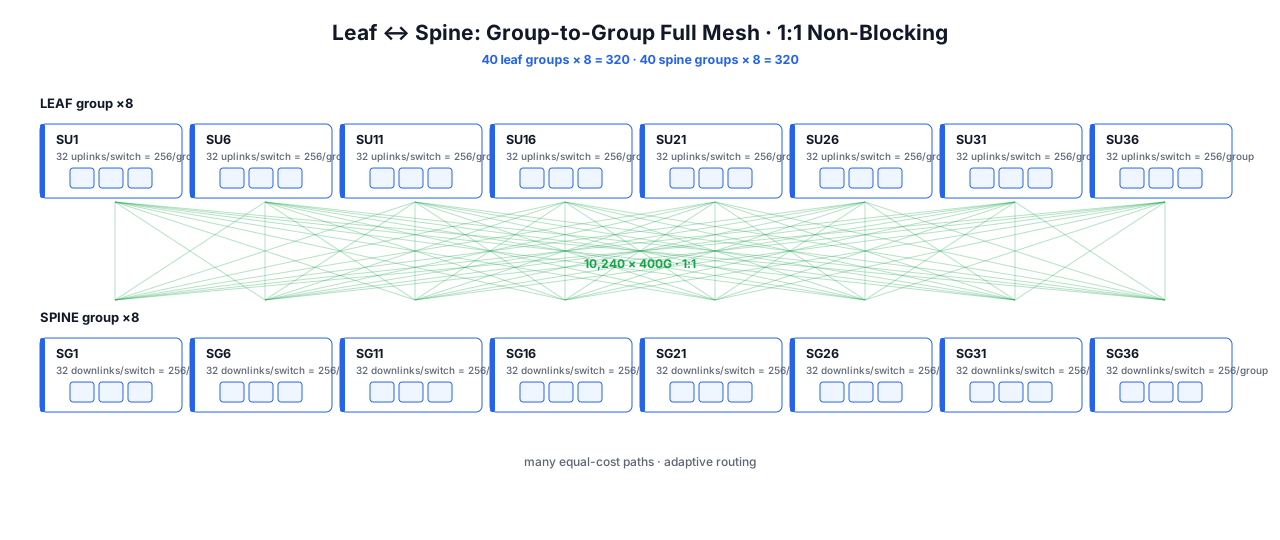
Each Leaf has 64 ports: 32 down to servers, 32 up to Spine. 40 Leaf groups × 8 × 32 = 10,240 uplinks; the Spine tier has 320 × 32 = 10,240 downlink ports — a group-to-group full mesh: each Leaf group's 256 uplinks spread across multiple Spine groups, so every Leaf has many equal-cost paths.

The Spine's value is horizontal bandwidth: intra-POD traffic (gradient exchange within a POD) mostly goes Leaf → Spine → Leaf without touching Core. This keeps most collective communication "local" — traffic localization is the invisible hero of a 10K fabric: more locality means lower end-to-end latency and a lighter Core tier.

5. Top Level: Spine ↔ Core — the Cross-POD Gate

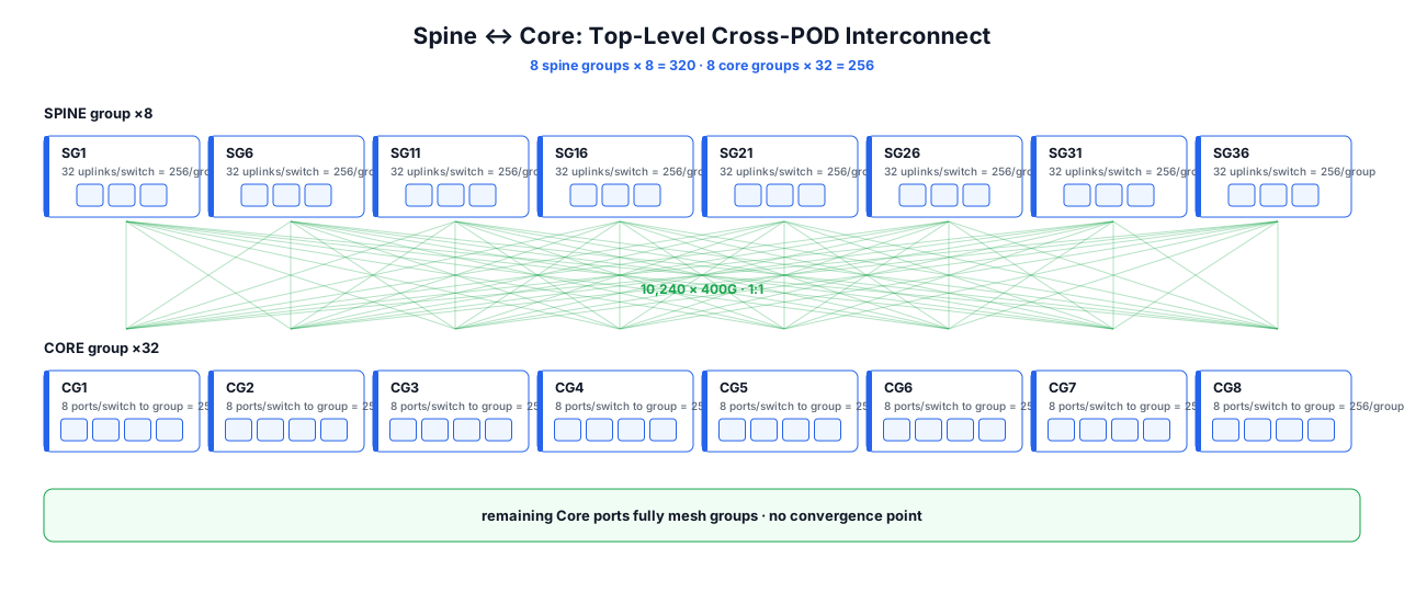
Cross-POD training (e.g., data-parallel gradient All-Reduce across POD1–POD5) must pass Core: Spine uplinks 320 × 32 = 10,240 → Core 256 × 40 = 10,240, again 1:1.

The 256 Core switches form 8 Core groups (CG1..CG8, 32 switches each). Core groups are fully meshed with the remaining ports, creating a top-tier non-blocking core: between any two PODs, no path has a convergence point.

6. Back to the Whole: A Cross-POD Packet's Full Journey

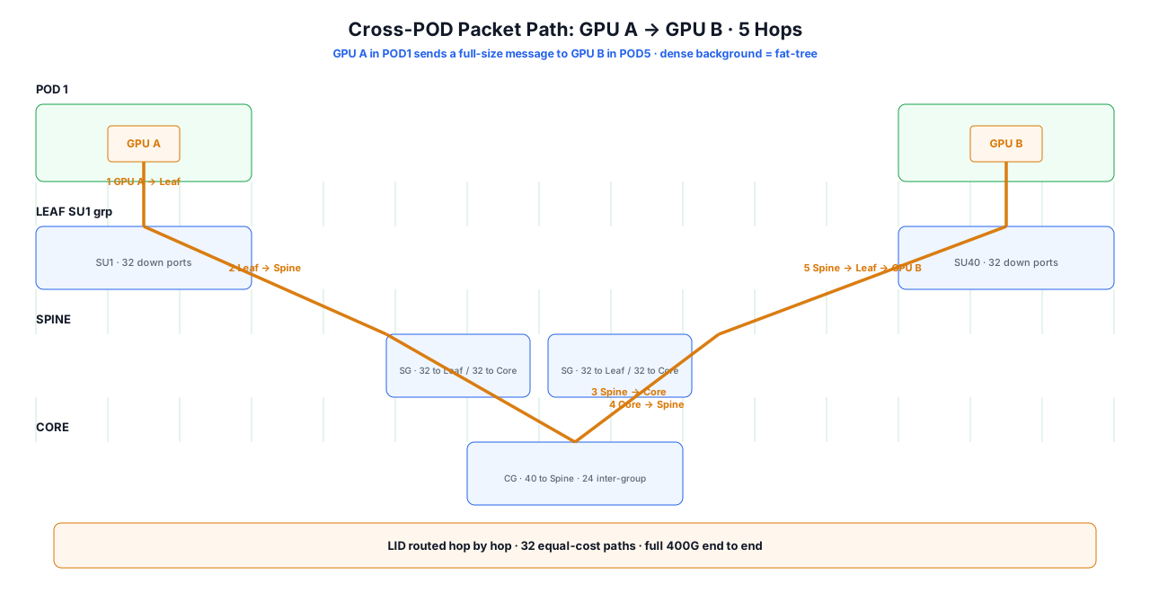
GPU A in POD1 sends a full-rate message to GPU B in POD5 — 5 hops:

1. GPU A → Leaf (SU1 group): the onboard ConnectX-7 pushes the message onto the 400G link;
2. Leaf → Spine: the Leaf looks up the LID routing table (installed by the SM) and picks an equal-cost uplink;
3. Spine → Core: cross-POD traffic goes up to a Core group;
4. Core → Spine → Leaf → GPU B: Core routes down to the target POD's Spine and Leaf, landing on GPU B's NIC.

5 hops, 1:1 bandwidth, zero loss (IB's link-layer credit flow control is lossless by design), latency kept minimal by LID routing + adaptive routing. To a training framework, this path is the physical carrier of a single NCCL All-Reduce.

7. Control Plane: UFM Dual Nodes and Subnet Management

• UFM (Unified Fabric Manager) ×2: the two UFM servers monitor the whole fabric — stats, performance, fault location; one fails, the other takes over, the control plane never stops.
• Subnet Manager (SM) primary/backup: exactly one master SM assigns LIDs and computes routes; at 10K scale, run SM together with UFM for second-level route convergence.
• PKey partitioning: compute and storage (IPoIB) use different PKeys, keeping training traffic isolated from other flows.
• SHARP in-network aggregation: QM9790 supports SHARP — part of All-Reduce reduction happens inside the switch, cutting communication volume in half. This is the "hidden advantage" of 10K-scale IB.

8. Why IB, Not RoCE

Dimension	IB (this architecture)	RoCE
Losslessness	credit-based, lossless by design	needs PFC/ECN hop-by-hop
In-network compute	native SHARP	none (extra solutions)
Routing	SM-computed + adaptive routing	vendor-dependent
Operations	UFM unified monitoring	multi-vendor assembly
Fit	the choice for 10K-scale training	small/medium, Ethernet reuse

In one sentence: at 10K scale, IB's "lossless out of the box + in-network reduction + unified ops" drops engineering complexity by an order of magnitude.

9. Deployment Checklist

1. Port reconciliation: 10,240 available ≥ 10,000 attachments; 1:1 non-blocking at every tier;
2. POD planning: ≤ 256 nodes per POD, 8 Leaf groups covering 2,048 ports;
3. Control-plane isolation: SM/UFM dual nodes on out-of-band network, off the parameter plane;
4. Partitioning: PKey isolation for compute/storage; VL mapping prioritizing compute;
5. Full-path testing: NCCL allreduce / alltoall, including cross-POD long paths;
6. Worst-case acceptance: cross-POD All-Reduce bandwidth should be ≥ 90% of intra-POD.

Related reading: InfiniBand Performance Tuning for AI Training, GPU Training Network Troubleshooting, NCCL Test & Optimization.